Euler's Method Explained: Approximating Solutions to Differential Equations

Euler's Method Explained: Approximating Solutions to Differential Equations

What Is Euler's Method?

Euler's method is a first-order numerical technique used to approximate solutions to ordinary differential equations (ODEs) when an exact, closed-form solution is difficult or impossible to find. Named after the Swiss mathematician Leonhard Euler, who first introduced the technique in the 18th century, it remains one of the most widely taught numerical methods in calculus and differential equations courses today — precisely because it's simple enough to compute by hand, yet powerful enough to illustrate how every more advanced numerical method (like Runge-Kutta) actually works underneath.

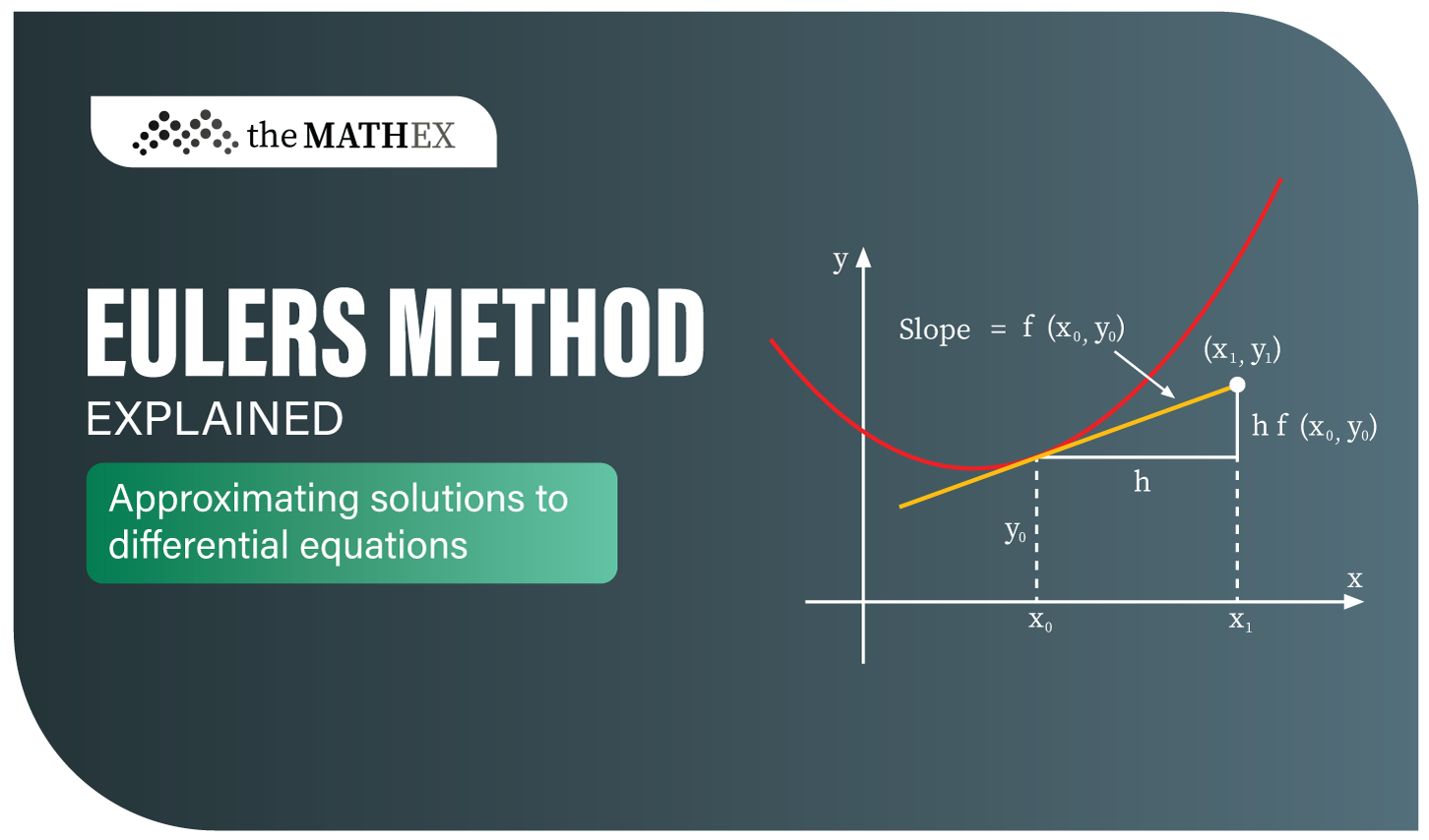
At its core, Euler's method takes a known starting point and a differential equation describing the rate of change at that point, then uses the slope of the tangent line to estimate where the solution curve goes next. Repeating this process step by step traces out an approximate path for a function whose exact formula may not be solvable using standard integration techniques.

The Euler's Method Formula

For a first-order initial value problem of the form:

dy/dx = f(x, y), y(x₀) = y₀

Euler's method estimates the next point on the solution curve using:

yₙ₊₁ = yₙ + h × f(xₙ, yₙ)

Here, h is the step size, f(xₙ, yₙ) is the differential equation evaluated at the current point, and yₙ₊₁ is the approximated value at the next x-value (xₙ₊₁ = xₙ + h). This process repeats iteratively, using each new approximation as the starting point for the next step.

How to Use Euler's Method: Step-by-Step

1. Identify the differential equation and initial condition. Write the ODE in the form dy/dx = f(x, y), and note the starting point (x₀, y₀).
2. Choose a step size (h). Smaller step sizes generally produce more accurate results but require more iterations to reach the target x-value.
3. Evaluate f(x, y) at the current point. This gives the slope of the tangent line at that location.
4. Apply the formula. Multiply the slope by the step size and add it to the current y-value to get the next approximation.
5. Repeat for each subsequent step. Continue until you reach the desired x-value, using each new (x, y) pair as the input for the next iteration.

Worked Example

Consider the initial value problem dy/dx = x + y, with y(0) = 1, and a step size of h = 0.5. We want to approximate y(1).

Step 1: At x₀ = 0, y₀ = 1. f(x₀, y₀) = 0 + 1 = 1. So y₁ = 1 + 0.5(1) = 1.5, at x₁ = 0.5.

Step 2: At x₁ = 0.5, y₁ = 1.5. f(x₁, y₁) = 0.5 + 1.5 = 2. So y₂ = 1.5 + 0.5(2) = 2.5, at x₂ = 1.

So Euler's method approximates y(1) ≈ 2.5. Comparing this against the exact solution of this particular ODE (y = 2eˣ - x - 1, which gives y(1) ≈ 3.44) shows the approximation carries noticeable error — a useful illustration of why step size matters so much in practice.

Why Step Size Matters: Accuracy and Error

Euler's method is classified as a first-order method, meaning the local error at each step is proportional to the square of the step size, while the accumulated global error is proportional to the step size itself. In plain terms: halving the step size roughly halves the overall error, but it also doubles the number of calculations needed. This trade-off between accuracy and computational cost is central to understanding when Euler's method is appropriate and when a more refined technique is warranted.

For problems requiring higher precision, mathematicians often turn to the Improved Euler's Method (Heun's Method) or the Runge-Kutta methods, both of which reduce error by sampling the slope at more than one point per step rather than relying solely on the starting slope. Euler's method remains valuable, though, because it's the conceptual foundation those more advanced methods are built on — understanding it thoroughly makes every subsequent numerical method easier to grasp.

Using an Euler's Method Calculator

Working through Euler's method by hand is manageable for a handful of steps, but real-world problems often require dozens or hundreds of iterations to reach a useful level of accuracy — at which point manual computation becomes tedious and error-prone. A dependable calculator should:

• Accept the differential equation, initial condition, and step size as direct inputs, without requiring manual rearrangement of the equation.
• Iterate automatically through each step, applying the formula consistently without arithmetic slips.
• Display a full table of intermediate values — not just the final answer — so the approximation process is transparent and verifiable at every stage.
• Allow the step size to be adjusted, so users can directly observe how a smaller h improves accuracy at the cost of more computation.
• Support a range of differential equations, including those involving exponential, trigonometric, and polynomial terms.

This transparency is what makes a calculator genuinely useful for learning, not just for getting an answer — seeing each iteration reinforces how the method actually works rather than treating it as a black box.

Real-World Applications

Euler's method isn't confined to textbooks. It's used in population growth and decay modeling, where continuous differential equations describe how a population changes over time. In physics and engineering, it approximates motion under variable forces when an exact solution isn't tractable. In finance, related numerical techniques model the evolution of interest rates and option prices. Its simplicity also makes it a common entry point for programming exercises, since implementing the iterative formula in code is often a student's first hands-on encounter with numerical analysis.

Common Mistakes to Avoid

• Using too large a step size. A large h can cause the approximation to drift significantly from the true solution, especially over many iterations.
• Miscalculating f(x, y) at each step. Since every iteration depends on the previous one, an early arithmetic error compounds through all subsequent steps.
• Confusing local error with global error. A method can look accurate at a single step while still accumulating significant error over the full interval.
• Applying it to equations Euler's method isn't suited for, such as stiff differential equations, where the method can become unstable regardless of step size.

Related Concepts Worth Understanding Together

• Runge-Kutta methods: higher-order techniques that build directly on the logic of Euler's method for improved accuracy.
• Initial value problems: the category of differential equations Euler's method is designed to solve.
• Numerical stability: why some equations require smaller step sizes or entirely different methods to approximate reliably.

Understanding the formula, walking through a worked example by hand, and then verifying results with a calculator that shows every iteration is the most effective way to build lasting intuition for numerical methods — a skill that carries directly into more advanced differential equations coursework and applied engineering work.